Tipoff Monte Carlo
This scenario exercises the provided MATLAB monte carlo scripts to demonstrate performing this type of analysis. The particular topic being covered is the initial tipoff from a launch vehicle. This simulation experiences randomized initial orientations, rates, and positions. The spacecraft will go through a sequence to perform attitude and ephemeris acquisition using the SunAcq mode. SunAcq is an attitude control mode designed to orient the spacecraft in a power-positive orientation without requiring a full attitude and ephemeris solution. In this mode, the control is wrapped around the Sun Sensors themselves.
There are several items provided in the ExampleScenarios directory that relate to this example:
| Directory or File | Description |
|---|---|
| C:\ProgramData\AGI\STK_ODTK 13\SOLIS | A directory where the simulation data (in time-stamped sub-dirs) will go for this example scenario. |
| SOLISExample_TipoffMonteCarlo_Analyze.m | A post-processing script to run after the monte carlo data has been collected. |
| SOLISExample_TipoffMonteCarlo_Input.xlsx | The monte carlo input spreadsheet which defines the randomized distributions. Monte carlo configurations are set AFTER the standard configuration and will override any standard settings. The last entry wins. |
| SOLISExample_TipoffMonteCarlo_MCResults_100RunSet.mat | A monte carlo output set of 100 runs saved to use as an example for the analysis scripts. Load this file into MATLAB to see it's IN and OUT. |
| SOLISExample_TipoffMonteCarlo_Process.m | The MATLAB script called after each simulation run to collect metrics for the run. This function is set to run using Inputs.PostRun_CustomFunctionCalls within SOLISExample_TipoffMonteCarlo_Run.m |
| SOLISExample_TipoffMonteCarlo_Run.m | This is the MATLAB script used to run the monte carlo. It can be used to run a new monte carlo set or to repeat runs from an old monte carlo set. |
Included file details
Monte Carlo simulation data
Upon completion of running SOLISExample_TipoffMonteCarlo_Run.m, you will find a set of time-stamped simulation data within the satellite's output telemetry directory (typically within the C:\ProgramData\AGI\STK_ODTK 13\SOLIS directory). The data directory contains the CSV file telemetry and a *.mat file (loadable within MATLAB) which can be used to rerun the simulation and evaluate it's inputs (IN) or outputs (OUT). The OUTs are computed within SOLISExample_TipoffMonteCarlo_Process.m.
SOLISExample_TipoffMonteCarlo_Analyze.m
>> SOLISExample_TipoffMonteCarlo_Analyze('SOLISExample_TipoffMonteCarlo_MCResults_100RunSet.mat'); Run plot metrics on the example set.
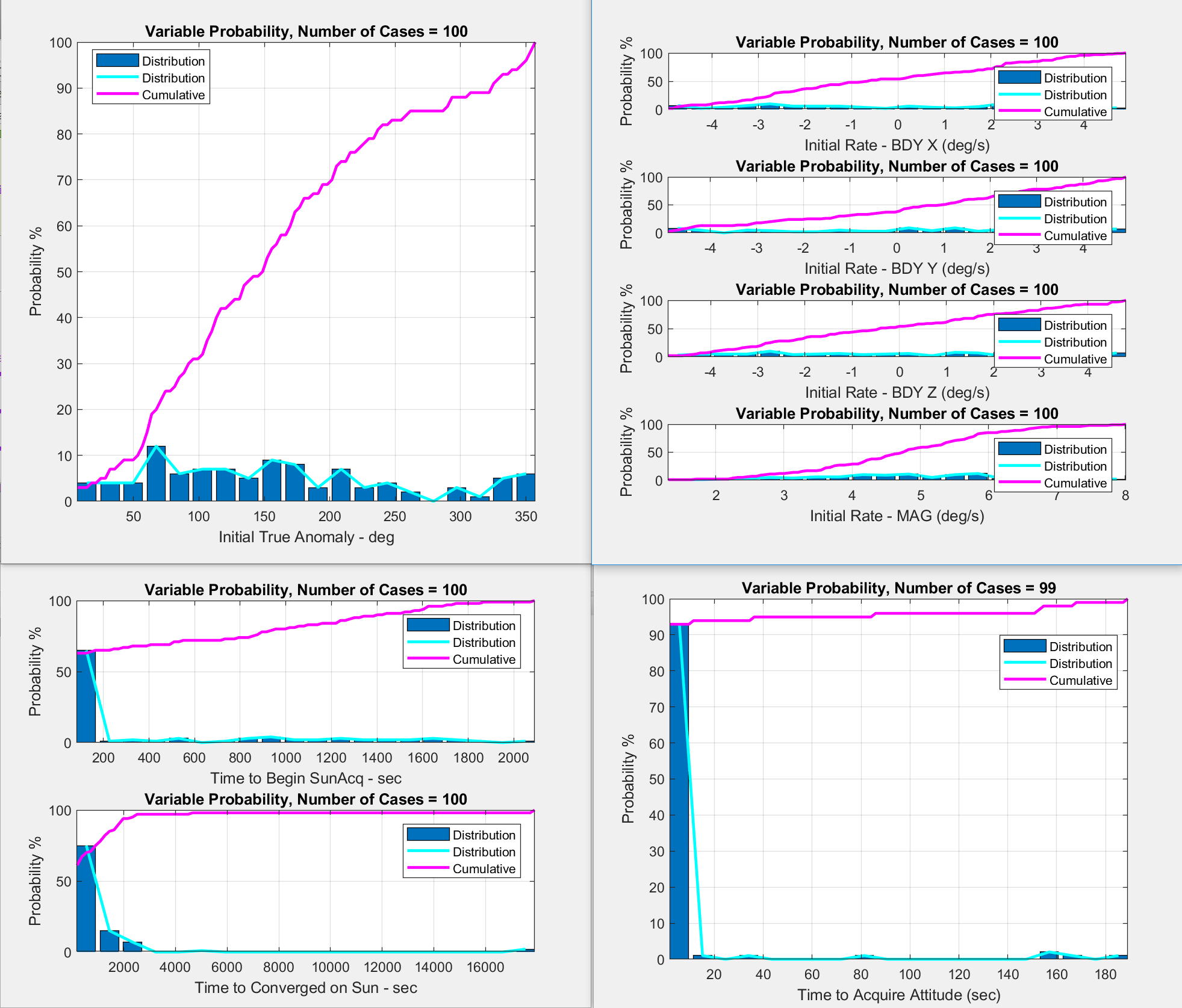
In the plots below, we see that the Initial True Anomaly resembles roughly a Uniform distribution (as we specified). We can also see that the initial spacecraft rates vary from -5 deg/s to +5 deg/s in each axis. Taking a look at the lower plots, we can see that ~60% of the runs begin SunAcq within the first 100 seconds with the 90th percentile occurring around 1600 seconds. In ~92% of cases, attitude is acquired almost immediately. For those that don't acquire attitude, it is likely that the star tracker is being blocked by the Earth, and the spacecraft is in eclipse. This should start to give a feel for the endless possibilities of analysis that can be completed via Automation.

SOLISExample_TipoffMonteCarlo_Input.xlsx
NominalPreCalibration Sheet
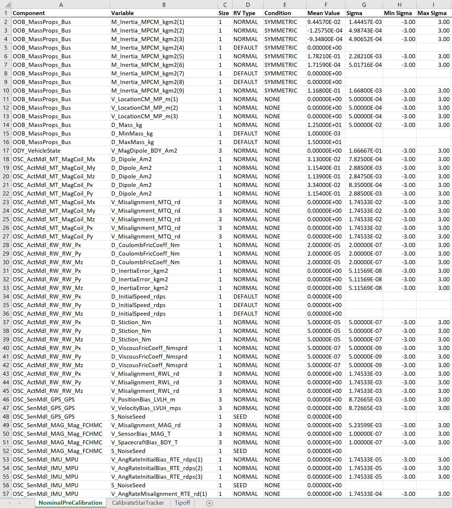
The first sheet that is called-out from SOLISExample_TipoffMonteCarlo_Run.m is "NominalPreCalibration". This sheet specifies randomization for vehicle inertia, cg location, actuator modeling parameters, and sensor modeling parameters.
Lets take a look at a few specific distributions:
-
Rows 2-10: Here we are randomizing the inertia tensor. If an inertia tensor was not symmetric, that would be a bad day for simulation. You will notice the Condition column is set to SYMMETRIC which will enforce that the Lower Left triangle of the matrix is equal to the upper right. Rows 5, 8, and 9 really aren't necessary here.
-
Rows 11-13 and 21: Here we are setting a VECTOR element in two different ways. In lines 11-13, we set each element of the VECTOR individually. This is useful if one axis of the VECTOR requires a different distribution than another axis. In line 21, the VECTOR distribution is done in one line by specifying a size of 3. In this case, all of the axes have the same distribution range (the draws are still independent per axis). Since lines 11-13 all specify the same distribution, they could have been done like line 21, but they are shown this way for demonstration purposes.
-
Row 14: This row is randomizing the mass using a NORMAL (Gaussian) distribution with a mean value of 12.5kg and a standard deviation of 0.05kg. The draws are constrained to fall between +/- 3-sigma. Any draw that falls outside the range will be redrawn until it fits (it does not simply get limited to the 3-sigma value).
| Random Variable Type | Description |
|---|---|
| DEFAULT | Draws a single value every time as-specified in the Mean Value column. Sigma, Min Sigma, and Max Sigma are not used. |
| UNIFORM | Draws a uniform distribution from Mean - Sigma to Mean + Sigma. Min Sigma and Max Sigma are not used, though sometimes -1 and 1 are specified. |
| NORMAL | Draws a normal Gaussian distribution from Mean - MinSigma * Sigma to Mean + MaxSigma * Sigma. If the draw falls outside the sigma range, it will be redrawn until it fits. |
| SEED | An integer value used to seed a random number generator. Mean, Sigma, Min Sigma, and Max Sigma are not used. |

Tipoff Sheet
The "Tipoff" sheet below is called after the "NominalPreCalibration" sheet above. Any items that exist in both sheets is overwritten by the result from the "Tipoff" sheet. Within this sheet, there are a few items listed as DERIVED under component. This is an indicator that the variable being randomized needs to be used to derive some other variable. In this case, the orbital elements are not direct inputs to the simulation, but Position, Velocity, and Time are. So, an Inputs.PreRun_CustomFunctionCalls(SOL_CustomInputFunction_SetOrbit) is setup from SOLISExample_TipoffMonteCarlo_Run.

SOLISExample_TipoffMonteCarlo_Process.m
This function is called from SOL_Run_MonteCarlo.m as part of a PostRun_CustomFunctionCall. PostRun functions are passed-in to SOL_Run_MonteCarlo.m in this manner to be used by the MATLAB eval function. By settings things up this way, we are able to keep SOL_Run_MonteCarlo.m entirely generic while providing you with customization ability to perform metric calculations on a run. This example computes multiple metrics, including but not limited to:
- Initial Rates
- Time to SunAcq
- Time to RateDamp
- EigenSlewDuration
- Pointing Errors
- Knowledge Errors
SOLISExample_TipoffMonteCarlo_Run.m
This is the main script that executes the simulation set. It can be used to execute a new monte carlo set or to repeat runs from a previous monte carlo set.
| Example Function | Description |
|---|---|
>> SOLISExample_TipoffMonteCarlo_Run(5);
|
Run a new set of 5 runs. |
>> SOLISExample_TipoffMonteCarlo_Run([22,41:43,86],'SOLISExample_TipoffMonteCarlo_MCResults_100RunSet.mat');
|
Repeat runs 22, 41, 42, 43, and 86 of a previously-run set. |